More `boRing` Examples

This vignette uses the penguins data set from the palmerpenguins package by Allison Horst, Alison Hill, and Kristen Gorman to demonstrate features of boRing.

# install.packages("palmerpenguins")
# install.packages("ggplot2")
library(palmerpenguins)
library(ggplot2)
library(boRing)

The penguins data frame contains observations about penguins consisting of year, species, sex, name of island where a bird was observed, and four physical measurements.

species	island	bill_length_mm	bill_depth_mm	flipper_length_mm	body_mass_g	sex	year
Adelie	Torgersen	39.1	18.7	181	3750	male	2007
Adelie	Torgersen	39.5	17.4	186	3800	female	2007
Adelie	Torgersen	40.3	18.0	195	3250	female	2007
Adelie	Torgersen	NA	NA	NA	NA	NA	2007
Adelie	Torgersen	36.7	19.3	193	3450	female	2007
Adelie	Torgersen	39.3	20.6	190	3650	male	2007

Note that there are missing values for some observations.

If we plot the body mass of penguins versus their flipper length, we can observe some clustering by species.

penguins |>
  ggplot(aes(x = flipper_length_mm, y = body_mass_g, color = species)) +
  geom_point(size = 1) +
  scale_color_brewer(palette = "Dark2") +
  guides(color = guide_legend(position = "top")) +
  theme_bw(base_size = 7) +
  theme(
    legend.title = element_blank()
  )
#> Warning: Removed 2 rows containing missing values or values outside the scale range
#> (`geom_point()`).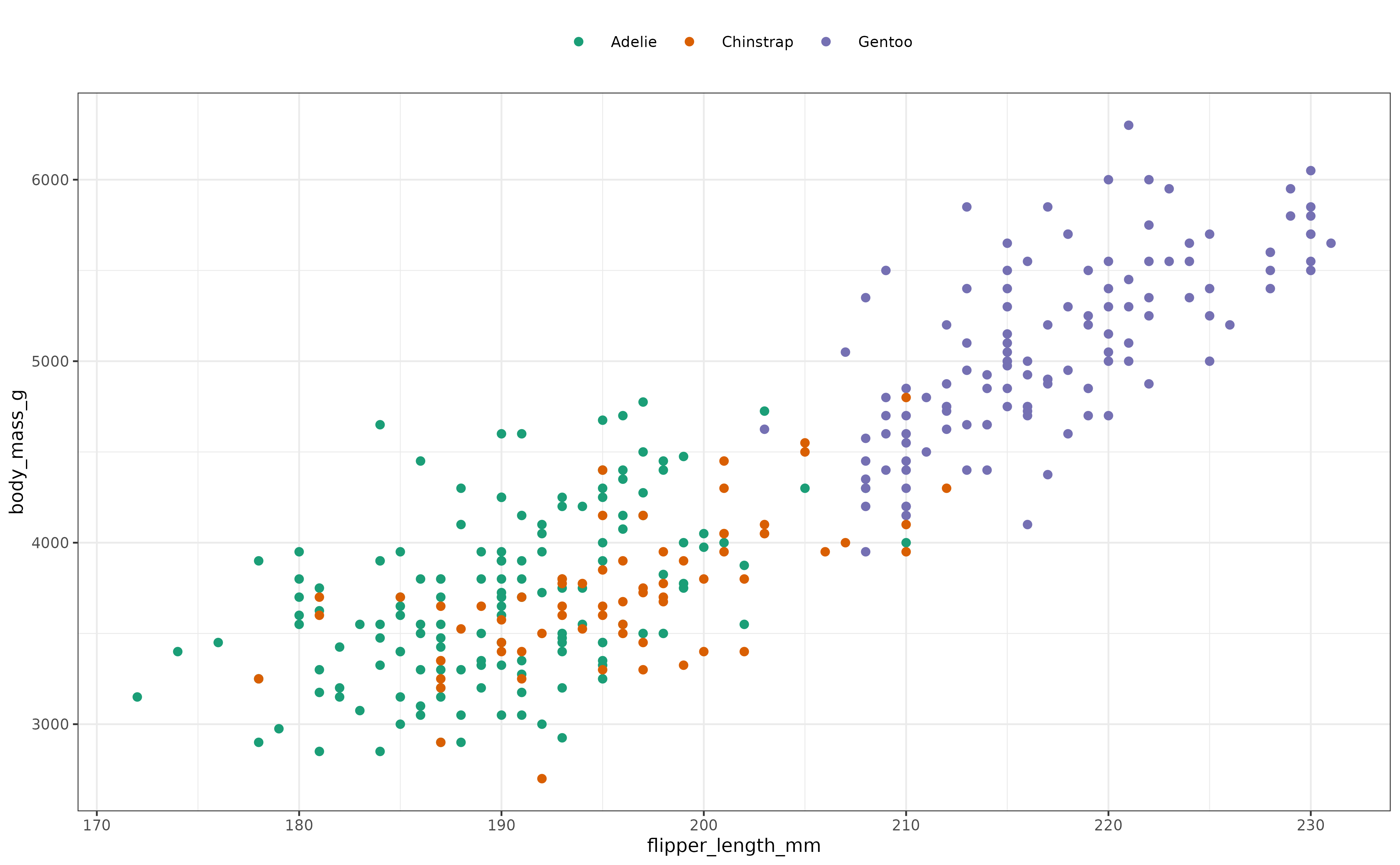

This data appears to lack unimodality. Let’s compute the boringness index for the plotted data:

penguins |>
  dplyr::select(flipper_length_mm, body_mass_g) |>
  as.matrix() |>
  boring(na_rm = TRUE, conf_level = 0.95)
#>  estimate  lower_ci  upper_ci 
#> 0.2271832 0.1241233 0.3253939

The boringness index value reflects what we observed in the plot. Contrast the previous result with the boringness index value obtained when we restrict to only the Gentoo species:

penguins |>
  dplyr::filter(species == "Gentoo") |>
  dplyr::select(flipper_length_mm, body_mass_g) |>
  as.matrix() |>
  boring(na_rm = TRUE, conf_level = 0.95)
#>  estimate  lower_ci  upper_ci 
#> 0.8290167 0.7641294 0.8772953

This boringness index value is consistent with the increased unimodality of the data when observing only the single species of Gentoo.

As another illustration, let’s examine the relationship between the bill length and bill depth of the penguins:

penguins |>
  ggplot(aes(x = bill_length_mm, y = bill_depth_mm, color = species)) +
  geom_point(size = 1) +
  scale_color_brewer(palette = "Dark2") +
  guides(color = guide_legend(position = "top")) +
  theme_bw(base_size = 7) +
  theme(
    legend.title = element_blank()
  )
#> Warning: Removed 2 rows containing missing values or values outside the scale range
#> (`geom_point()`).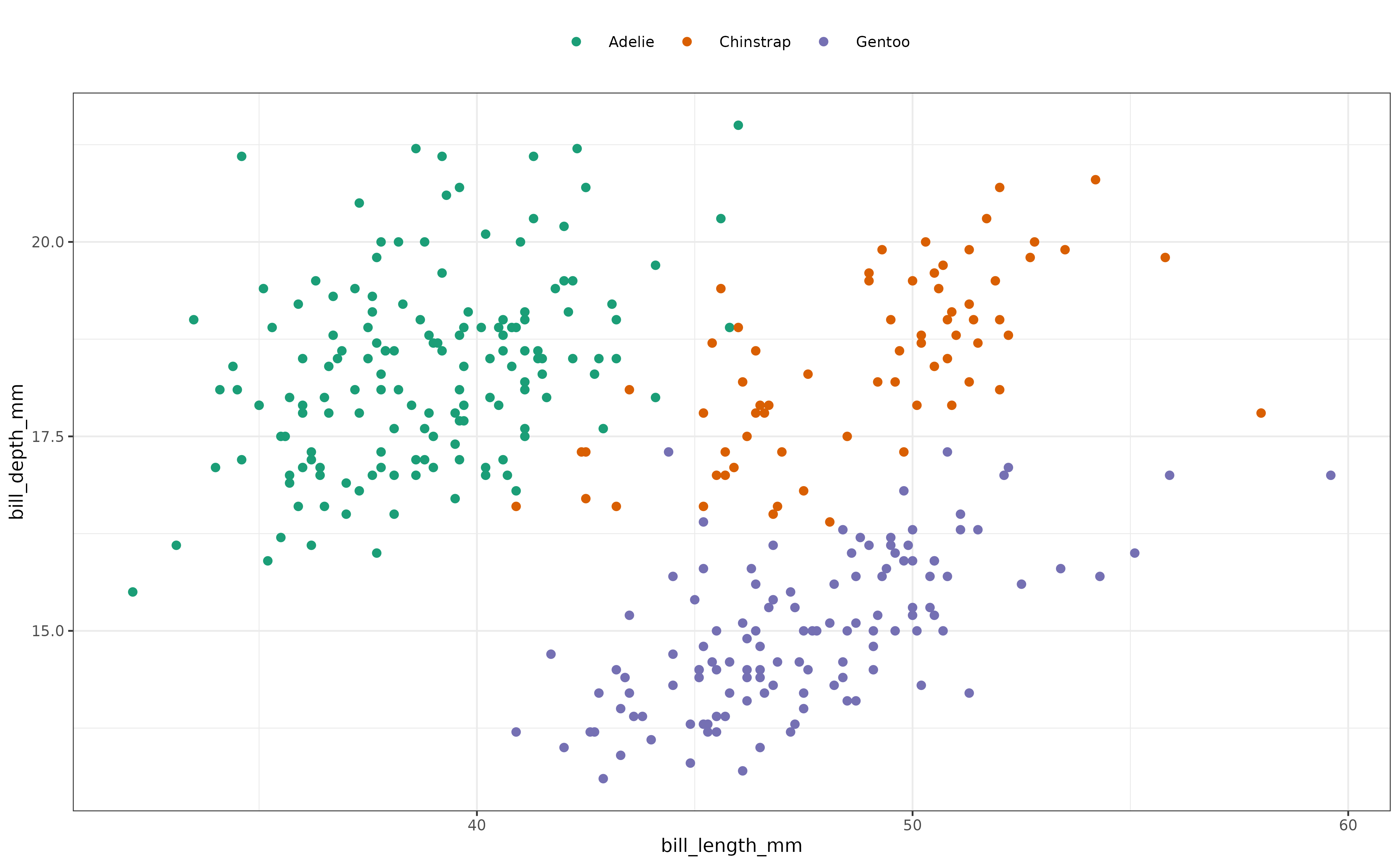

Again, this data appears to lacks unimodality but now there is also lower density in the center of the cloud of data points. Let’s compute the boring metric for the plotted data:

penguins |>
  dplyr::select(bill_length_mm, bill_depth_mm) |>
  as.matrix() |>
  boring(na_rm = TRUE, conf_level = 0.95)
#>    estimate    lower_ci    upper_ci 
#> -0.20111434 -0.30075022 -0.09713572

The negative value for the boringness index is consistent with what we observed in the plot.

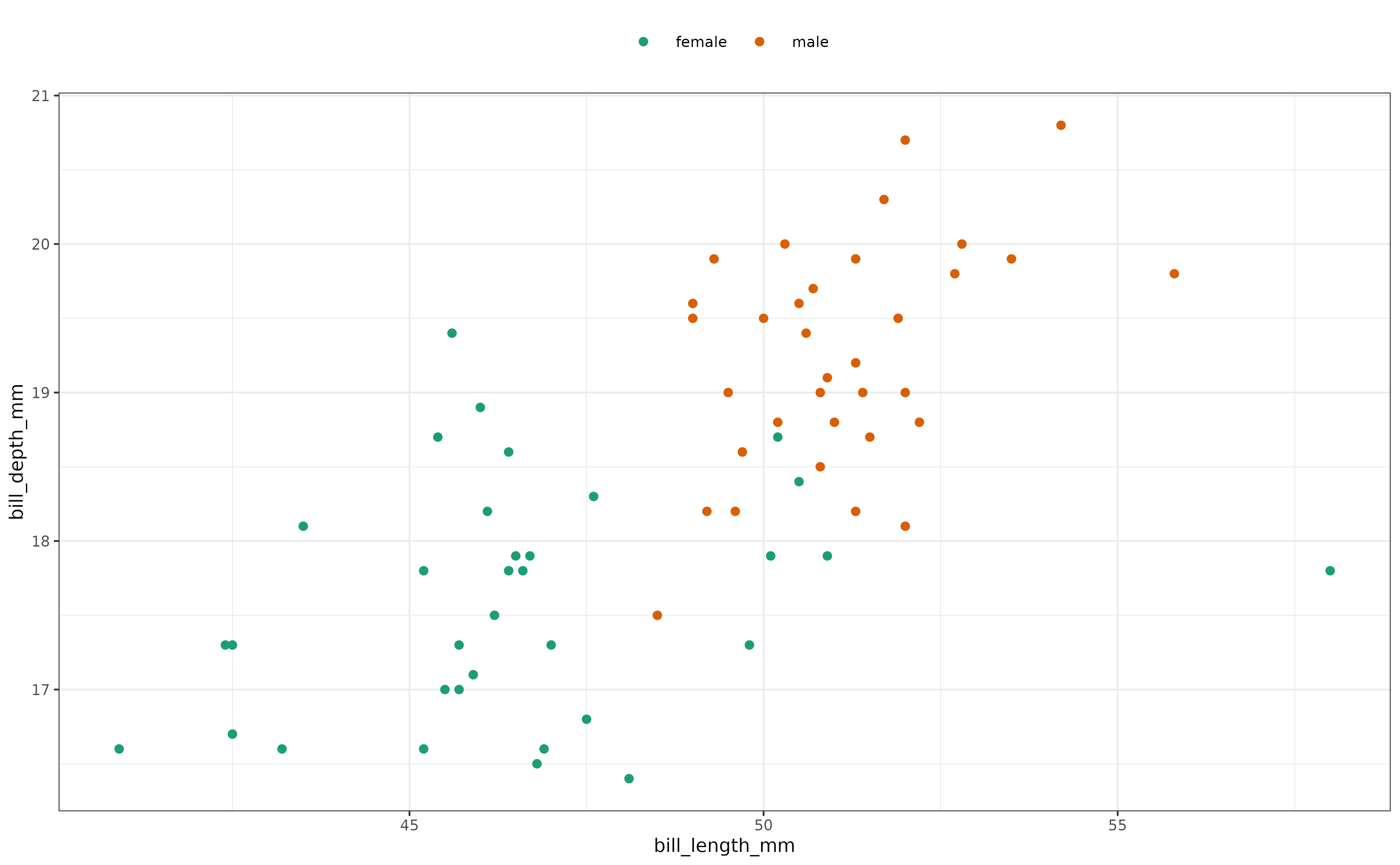
It may be interesting to consider what is happening with regard to the bill length and bill depth for the Chinstrap species:

penguins |>
  dplyr::filter(species == "Chinstrap") |>
  dplyr::select(bill_length_mm, bill_depth_mm) |>
  as.matrix() |>
  boring(na_rm = TRUE, conf_level = 0.95)
#>  estimate  lower_ci  upper_ci 
#> 0.6132763 0.4390492 0.7430520

A relatively low value of unimodality is predicted. This may be explained looking at the difference in the measurements across sex:

penguins |>
  dplyr::filter(species == "Chinstrap") |>
  dplyr::select(bill_length_mm, bill_depth_mm, sex) |>
  ggplot(aes(x = bill_length_mm, y = bill_depth_mm, color = sex)) +
  geom_point(size = 1) +
  scale_color_brewer(palette = "Dark2") +
  guides(color = guide_legend(position = "top")) +
  theme_bw(base_size = 7) +
  theme(
    legend.title = element_blank()
  )

Finally, we compute the boringness index for all four physical measurements:

penguins |>
  dplyr::select(bill_length_mm, bill_depth_mm, body_mass_g, flipper_length_mm) |>
  as.matrix() |>
  boring(na_rm = TRUE, conf_level = 0.95)
#>  estimate  lower_ci  upper_ci 
#> 0.6469143 0.5807034 0.7046236

Jason M. Graham

Simon Garnier

2024-05-10